You can enter formulas into the cells in a worksheet. These formulas can reference cells in different worksheets, working rows or comparison rows. Rather than including more complex spreadsheet functions, Budgets and Forecasts keeps a level of simplicity by allowing for basic arithmetic in these formulas.
Enter a basic formula
You enter formulas in a similar way to how you do it in other spreadsheet software, such as Microsoft Excel or Google Sheets, either directly into a cell or in the fx (formula) bar at the top of the grid when the cell is selected.
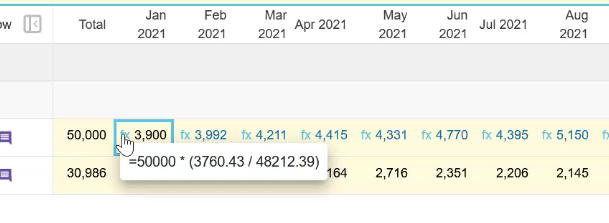
It is easy to identify and understand formulas in Budgets and Forecasts. When a cell contains a formula, the cell value has a blue fx indicator next to it. You can hover over this indicator to view the formula or click a cell and view the formula in the fx bar.
Use operators
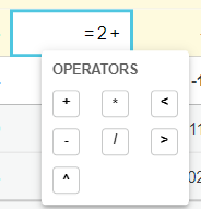
When you enter or edit an operator in a formula, a list of available operators displays. You can either use this list as a reference, so you know which operators you can use, or click the required operator to insert it into the formula.
Reference other cells in formulas
To enter more advanced formulas, you can reference values in other cells in the same worksheet (including those in comparison, sum and working lines) and in other worksheets (such as driver tabs).
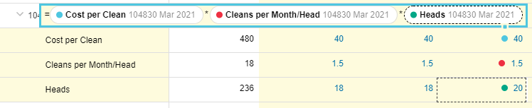
When you view a formula in the fx bar, a description of the referenced cells display, along with a colored dot corresponding to those cells. So you can easily see what you’re calculating, rather than just a reference to a cell number.
| Info |
|---|
When you copy and paste cells that contain formulas, you can control how those formulas behave. In the majority of cases, the cell references are relative by default but you can switch to absolute references, if required. See the Copy and paste formulas (relative v absolute references) section below. |
The following examples might be useful in your budget or forecast worksheet.
| Expand | ||
|---|---|---|
| ||
Your IT Computer Costs are a function of wages. In the formula below, the IT costs are 2% of AU wages. 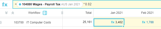 |
| Expand | ||
|---|---|---|
| ||
You added a Manual Entry Driver tab (which is named Assumptions) in which you entered an AUD exchange rate. You want to use that rate to calculate the budgeted cost of the Australian Conference. In the formula below, the Conference - AUD value is multiplied by the exchange rate in the Assumptions tab. 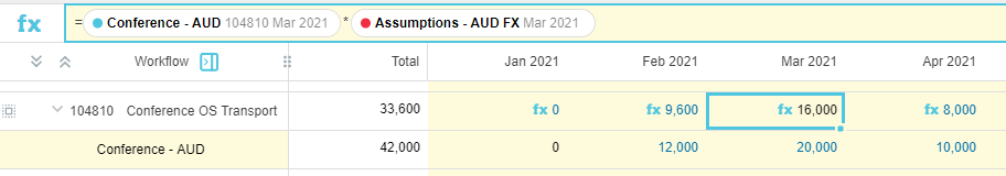 |
| Expand | ||
|---|---|---|
| ||
You want the Sales budget values for this year to be ten percent higher than last year’s actuals. In the formula below, the April 2021 sales value is made up of the actual value from 2021 plus ten percent. 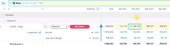 |
Use functions in formulas
You can use several different functions in your formulas. The available functions are listed below (in alphabetical order). Expand each section to view a description and example.
Enter a function
You enter functions in the same way you do in other worksheet software. The general steps are as follows:
Select the cell in which you want to enter the function.
Press the Equals '='key to indicate that you're entering a function.
Start typing the name of the function you want to use. As you type, a list of function names displays based on what you've entered so far.
Select the required function from the list (or continue typing the function name).
Press the Open parentheses '(' key to indicate the beginning of the function's arguments, which are the cells of data on which the function operates.
Select the arguments (reference cells). You can separate multiple arguments with commas or use your keyboard to select a range of arguments.
See Use a range in a function below for more information.
See the SUM function section below for examples of the different ways to select the arguments.Press the Open parentheses ')' key to indicate the end of the function's arguments.
Press Enter or Return to complete the function entry. The result of the function displays in the cell where you entered it.
(Optional) Switch to absolute or relative references, if required.
| Anchor | ||||
|---|---|---|---|---|
|
You can reference a range of cells in functions. In most cases, the ranges can only be on a single row. For example, you can SUM across a row but not down a column.
Functions that accept cell ranges are:
SUM, MIN, MAX and AVERAGE. You can use the Shift+Arrow keys to select the range.
DAYS, WEEKDAYS, WORKINGDAYS and WD. Currently, you can only select a range for these functions using the mouse method (not via the keyboard).
See the SUM function section below for examples of the different ways to select a range of cells.
Learn about the functions
| Expand | ||
|---|---|---|
| ||
Function: ABS(value) Description:
Example: ABS(-2) = 2 |
| Expand | ||
|---|---|---|
| ||
Function: AVERAGE(value1, [value2...]) Description:
Example 1: AVERAGE(Jul 2025 .. Dec 2025) returns the average of the range from July 2025 to December 2025. Example 2: AVERAGE1, 2, 3) returns the average of 1, 2 and 3, which is 2. |
| Expand | ||
|---|---|---|
| ||
Function: DAYS Description:
Example 1: DAYS(Jun 2024) returns the number of days in June 2024. Example 2: You can refer to the other cells in the formula to calculate the number of days in a date range. Enter the function and within the parameters, select the cells that contain the values you want to include. DAYS(Jul 2025 - Dec 2025) returns the number of days in the range from July 2025 to December 2025. Example 3: Watch this video to learn how to use the days functions to calculate the number of days in a specified date range. |
| Expand | ||
|---|---|---|
| ||
Function: FINITE(value, result) Description:
Example 1: A common use case is to return a specific value of a formula that is divided by zero, for example, by returning a zero value rather than the #DIV/0! reference. FINITE(1/0, 0) returns the specified value of 0 instead of the #DIV/0! reference. Example 2: FINITE(-1/0,1,2,3) returns the value 2 as that was what was defined for -infinity, instead of the #DIV/0! reference. Other examples: FINITE(NaN, 0) = 0 FINITE(1/0, 5) = 5 |
| Expand | ||
|---|---|---|
| ||
Function: IF(logical expression, value if true, value if false) Description:
Example 1 - Basic IF function: IF(Sales > 7000000, Sales * 0.05, 0) If Sales are greater than 7 million, 5% of the Sales will be returned, else 0 will be returned. Example 2 - Nested IF function: If Sales are greater than 7 million, 5% of the Sales will be returned, else if Sales are greater than 1.2 million, 2% of the Sales will be returned, else 0 will be returned.  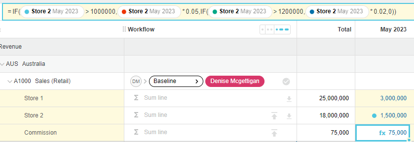 |
| Expand | ||
|---|---|---|
| ||
Function: MIN(value1, [value2...]) Description:
Example 1: MIN(Jul 2025 .. Dec2025) returns whichever has the smallest number out of the range from July 2025 to December 2025. Example 2: MIN(-2, 5, 10) returns -2 as that is the smallest number out of -2, 5, and 10. |
| Expand | ||
|---|---|---|
| ||
Function: MAX(value1, [value2...]) Description
Example 1: MAX(Jul 2025 .. Dec 2025) returns whichever has the largest number out of the range from July 2025 to December 2025. Example 2: MAX(-2, 5, 10) returns 10 as that is the largest number out of -2, 5, and 10. |
| Expand | ||
|---|---|---|
| ||
Function: POWER(base, exponent) Description:
Example: POWER(5,2) The number returned when 5 is raised to the power of 2 is 25. |
| Expand | ||
|---|---|---|
| ||
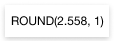
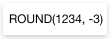
Function:ROUND(value, places) Description:
Examples:
|
| Expand | ||||||
|---|---|---|---|---|---|---|
| ||||||
Description:
Example 1: SUM(Jul 2025 .. Dec 2025) returns the sum of the range from July 2025 to December 2025. Example 2: SUM(Jun 2023, Jul 2023) returns the sum of the June 2023 and the July 2023 cells. Example 3 - Select cells in a range one at a time: Use a comma between each selected value, such as SUM(1,2,3) = 6. In the following example, the value in cell FL > Sep 2002 is the sum of the values in FL > Oct 2022, FL > Nov 2022 and FL > Dec 2022. In other words, 881 = 421 + 60 + 400. 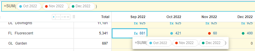  Example 4 - Select a range of cells using keyboard shortcuts: Use your keyboard to select a range of cells. Select the first cell in the range then either:
In the following example, the value in cell FL > Sep 2002 is the sum of the values in FL > Oct 2022 : Dec 2022.  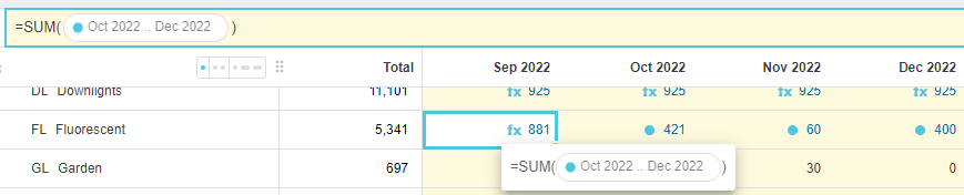 Example 5 - Select cells in a range (multiple methods): Watch this video… |
| Expand | ||
|---|---|---|
| ||
Function: SQRT(value) Description:
Example:SQRT(4) returns the square root of 4 is 2. |
| Expand | ||
|---|---|---|
| ||
Function: WEEKDAYS Description:
Example 1: WEEKDAYS(Jun 2024) returns the number of weekdays in June 2024. Example 2: WEEKDAYS(Jul 2025 - Dec 2025) returns the number of weekdays in the range from July 2025 to December 2025. |
| Expand | ||
|---|---|---|
| ||
Function: WORKINGDAYS(id, columns) Description:
Example 1: WORKINGDAYS(Working Days UK, Jun 2024) returns the number of working days in the month of June 2024 based on the Working Days UK calendar. Example 2: WORKINGDAYS(Working Days UK, Jul 2025 - Dec 2025)returns the number of working days in the range from July 2025 to December 2025 based on the Working Days UK calendar. |
Copy and paste formulas (relative v absolute references)
To save time, you can copy and paste formulas. When you copy a formula, the pasted formula might have an absolute or relative reference, depending on the situation, as outlined below. You can quickly switch between these reference types to meet your formula needs.
Use relative referencing
With relative referencing, the cell references adjust automatically in the target cell. In other words, the references change when the formula is copied into other cells, relative to the position (row and column) of the formula.
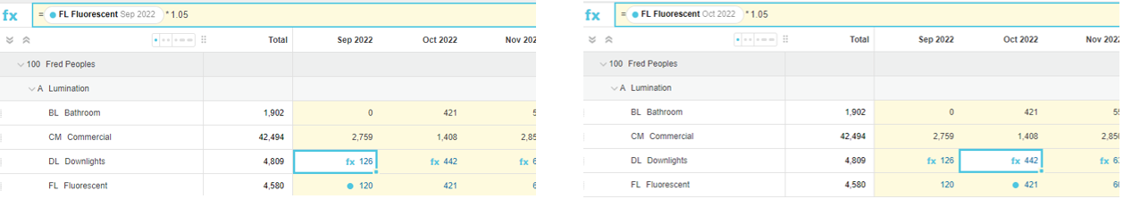
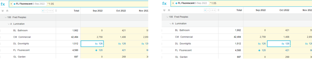
In the following example, the formula in DL > September 2022 cell references the value in the FL > September 2022 cell. When that formula is copied into the next cell, the reference is relative (the month changes), so the reference part of the formula changes to become FL > September 2022.
When you copy formulas in a budget or forecast worksheet, the cell references in the target cells are relative by default in the following situations:
When you use the copy forward feature. For example, if a cell references January data, when you copy the cell to February, it will reference February data.
When you copy a formula that references a comparison row. This applies both to formulas copied to the same row and to different rows from the original cell.
When you copy a formula that references a working row. For example, if the original cell has two working rows and a formula references both of those rows, copying the formula to a cell which has two or more working rows will result in a relative formula being pasted into the target cells. The target cells need to have the same working row offset.
When you copy a formula that references a cell in one level into a target cell in a different entity in the same level. For example, if you copy a formula in Branch A’s Cost of Goods Sold, which references sales in Branch A, and paste it into Branch B’s Cost of Goods Sold, the formula will reference to Branch B’s sales.
Use absolute referencing
With absolute referencing, the cell references are locked. In other words, the references do not change when the formula is copied into other cells.
When you copy formulas in a budget or forecast worksheet, the cell references in the target cells are absolute by default in only one situation; when you copy forward a cell in the Total column, i.e. the formula will always reference the total.
You can change the default relative references listed above to absolute references (see next section below). Following on from the example above, if you manually switch to absolute referencing, you can see the dollar sign in the formula denotes the absolute reference and the reference part of the formula is the same in both cells; FL > September 2022.
| Anchor | ||||
|---|---|---|---|---|
|
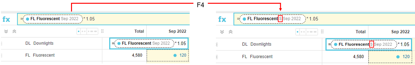
To switch (toggle) between absolute and relative references, in both a single cell reference and the components of a range, you use the F4 key.
Enter the formula into the required cell, then in the formula bar, select the reference element of that formula.
Press F4. A dollar sign displays next to the element (date) in the formula to identify it is an absolute reference.
Click out of the formula bar and press Enter to view your changes.
Copy the formula as required and note how the values change.
| Expand | ||
|---|---|---|
| ||
In the image below, the formula uses a function that references a range of cells. That formula was copied forward into the other cells in the row. By default, relative referencing applies. When you press F4 to switch to absolute referencing, the reference to the first cell in the range becomes absolute, as illustrated in the second image below. Note the difference in the values in the subsequent cells. 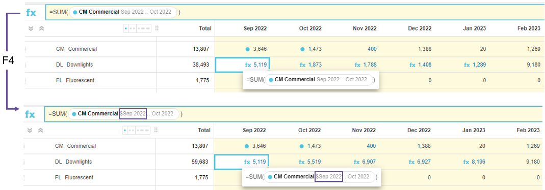 If you press F4 again (2nd time), all the references become absolute, as illustrated in the image below. 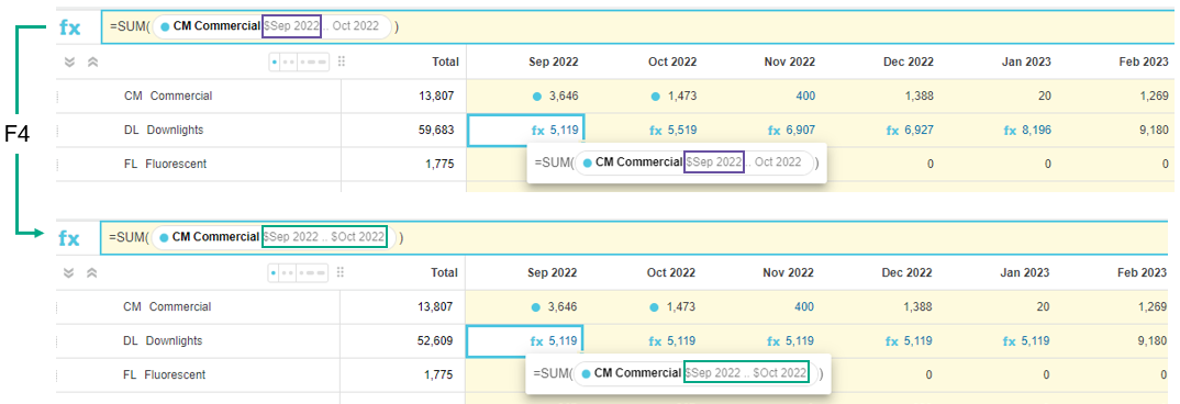 If you press F4 again (3rd time), the reference to the other cells in the range become absolute, as illustrated in the image below. 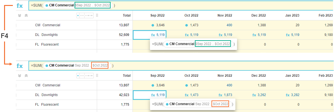 If you press F4 again (4th time), you return to how you started; relative referencing applies again. So you can quickly switch between the different types of referencing to control how the values are copied into the other cells. |
| Expand | ||
|---|---|---|
| ||
On this page
| Table of Contents | ||||||||||
|---|---|---|---|---|---|---|---|---|---|---|
|